Session 4

Map drawing continued

In this next exercise we will start making good use of the intelligence of vector data. Because of the rising water level, part of the Ancient Natural Woodlands is lost, we will have to replant some. We also have permission to plant a conifer plantation.

Open the project ‘My First Map’ (if not already on screen).

Save this project as…and type in the following new name: ‘My first map-Session 4’

5 DRAWING the map

5.1 Set up a new style

To map these new woodlands we need pencils to colour these in. In jargon: we first need to create two new styles in the style editor. Woodlands are usually shown in shades of green with trees symbols showing in them.

We have created new polygon entries before, so in short:

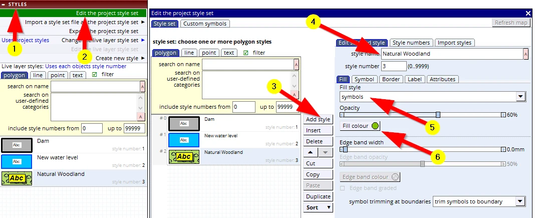
(1 –3) create a new polygon style entry:

(4) and name it ‘Natural Woodland’

(5) But what will be new is that we will now select Fill style: symbols Below it is the “Opacity” slider, set it to 50%

(6) Change the colour to a medium bright green

Keep this menu open,

then:

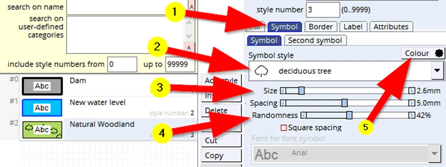
(1) Click on the Symbol tab

(2) Click on the Symbol style entry (or that black down arrow), scroll down and select: deciduous tree

(3) Reduce the default Size to about 2.5mm

(4) Increase the Randomness to about 40%

(5) Change the Colour to dark green if you want

Keep this menu open, then:

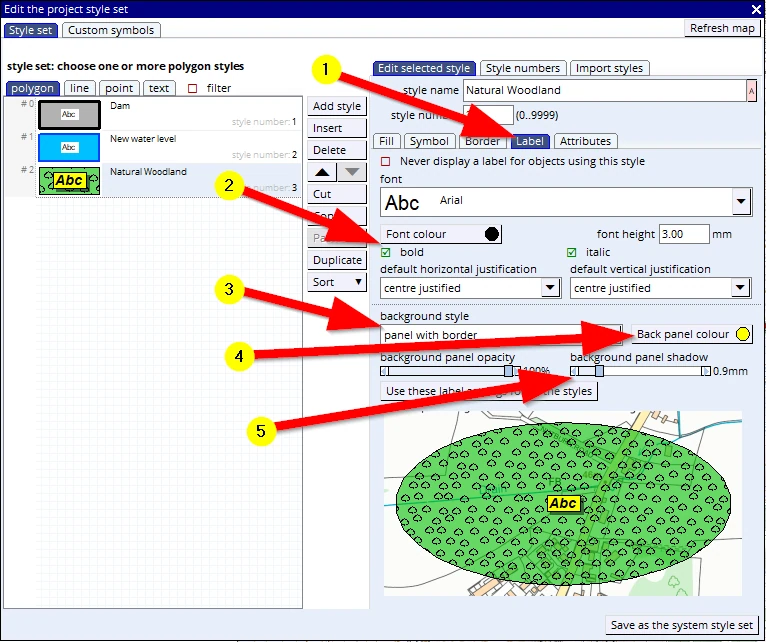
(1) Click on the Label tab

(2) Adjust any of these font settings to your liking (we’ll use ‘Arial’, 3mm, bold & italic)

(3) Change the background style to panel with border

(4) Change the Back panel colour to yellow.

(5) Change the background panel shadow to about 0.9 mm

Keep this menu open, but press ‘F1’ to save the project (and thus save these changes in the style file).

Keep this menu open, then:

Because this is a ‘Natural Woodland’ it will not be fenced off, so we don’t want to show a border around the area to be planted:

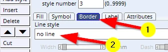
And because there is no fence around it, trees will grow beyond the polygon we will draw.

We can suggest that is happening with the following setting:

(1) Open the Fill tab

(2) choose the option let symbols spill over boundary

(3) note the resulting effect

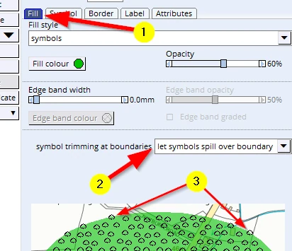
Keep this menu open, but do a F1 to save this project (and thus the changes made to this style).

As above, create a new style entry and call it ‘Conifer Plantation’.

(1-4) Choose a darker green fill colour and change the fill type to ‘Symbols’ - as done above). Set the opacity to 50%.

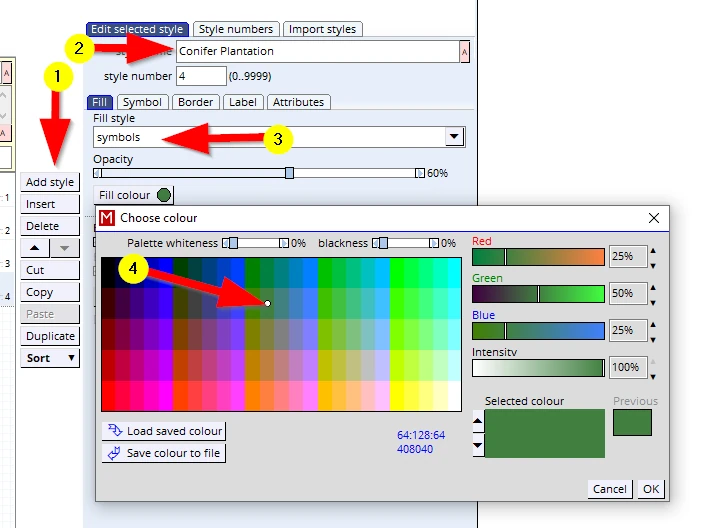
This style will also have trees as an infill pattern:

1. (1)This time select a coniferous tree symbol and change these settings:

Size to 1.8mm, Spacing to 3.0mm, leave the ‘Randomness’ slider on 0%

1. (2)Tick the box Square spacing
2. (3)This woodland will be fenced and so we will leave this setting as is.

In this case we shall leave the label settings as they are.

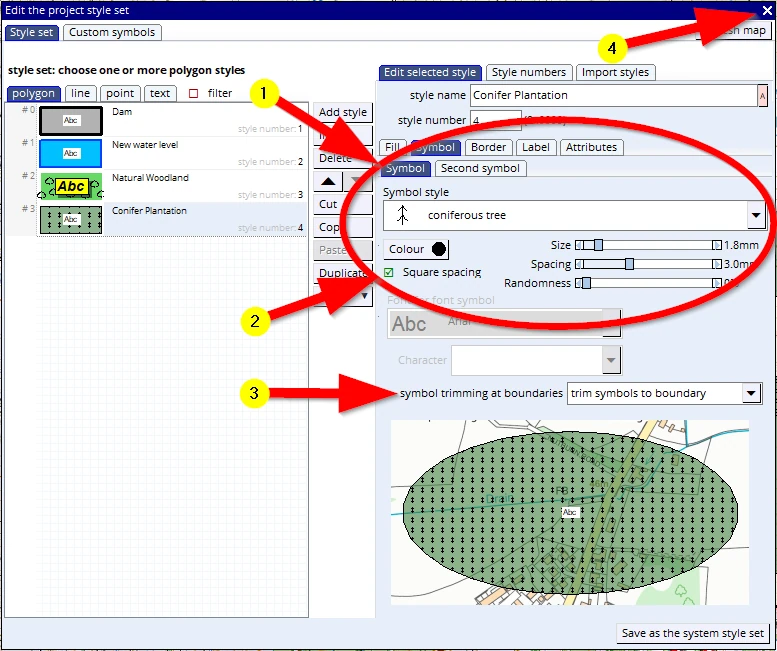
(4) Save your project (F1), and we can now close this menu by clicking on the little white cross.

We are now ready to actually draw these new woodlands.

Just in case you have some test polygons on screen, clear the live layer first:

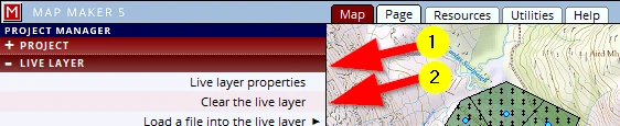
(1) LIVE LAYER header

(2) Clear the live layer

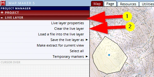
5.2 Drawing a polygon (using the Polygon tool)

Let’s start with the conifer plantation. It will be well fenced with long straight boundaries. For that reason the regular POLYGON tool is the best tool to use.

(1) Activate the POLYGON tool

(2) Digitise a shape which looks pretty much like this:

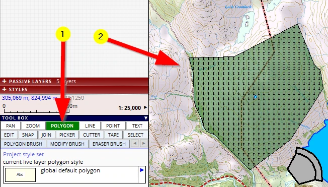
After we have closed the polygon the NEW POLYGON menu will open on the left.

(1) Assign the ‘Conifer Plantation’ style to it in the DEFAULT STYLE header.

(2) Open the ATTRIBUTES header

As explained, with vector data we can record all sorts of information in map objects. Currently we will only introduce a unique Identifier (ID).

The ATTRIBUTES header will have opened:

(1) Type in a unique ID for this woodland, ‘1’.

(2) Note what else the software is recording

(3) Confirm new polygon and finish edit

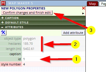
In the red LIVE LAYER header, save this layer in the Training folder and call it ‘Conifer Plantation_01’.

F1, to save your project.

5.3 Drawing a polygon (using the brush tool)

We will now ‘plant’ the Natural Woodlands. The layout has to have a ‘natural’ feel to it, there will be no fencing or straight hard boundaries, in other words, an ideal job for the ‘Polygon Brush’ tool.

For ease of work, please set the screen to about 1:25,000 scale.

Activate the POLYGON BRUSH tool and set it to about 15 pixels and draw a shape not bigger than the example below and in this location:

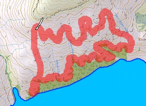
As soon as you let go of the mouse button the interface on the left changes to the NEW POLYGON menu.

(1) It will probably open on the ATTRIBUTE header because that was the last header we used please open the DEFAULT STYLE header

(2) Assign the ‘Natural Woodland’ style to this new object.

(3) Click on the CAPTION header.

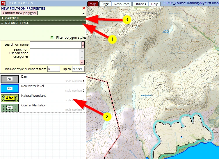
The CAPTION header opens and...

(1) We will name this woodland and give it, type in, the name ‘Yonder Wood’.

(2) Confirm new polygon and finish edit

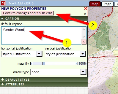
Perhaps you do not see the name on your screen. It depends on settings which we will explain in the section ‘Labels’ - don’t worry we will do that later!

We need to save this new layer:

(1) LIVE LAYER header

(2) Save the live layer as

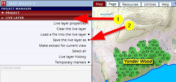
Browse to our usual folder and name it:

C:\MM_Course\Training\Natural Woodland_01

Follow it up with a ‘save project’ (F1)

Note: With the conifer plantation we typed in a specific ID. With the Natural Woodland we only typed in a specific name. We could have given both a name and ID, but we did not..

6 Working with LAYERS

When we draw or edit an object, we are doing that in a ‘live layer’. Saved layers become a ‘passive layer’.

When we select a layer and click on the little blue arrow (which then turns red) we open a new menu dealing with the most immediate actions possible. The actions speak for themselves: e.g. remove this layer, move layer up or down

And we have seen that more specific options can be accessed in the layer properties menu. This layer properties menu can also be found in the LIVE LAYER header.

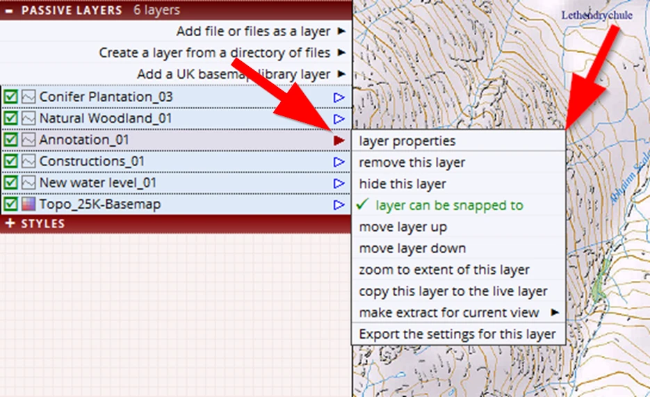
But why working with layers in the first place? After all, we can draw all and everything into one layer and be done with it.

There are 4 main reasons why we would want to split our work up into different layers. These are important reasons, so please take note.

1 Cartographic Effects

It gives us more flexibility in creating specific cartographic effects – we will use/demonstrate that later in this course

2 Ease of editing/working with map objects

It is easier to edit map objects. For example, we could draw a polygon first and then draw a symbol on top of it. But when it comes to editing, it then becomes a bit of a nuisance to edit the right object.

3 Management purposes

It is very likely that some of the map objects drawn for a specific map, can also be used in another project. Think of for example a layer with all ‘Public Rights of Ways’ (PRoWs). This is a layer which we can most likely use in another map as well. If however all sorts of other information is also drawn in the map and we wanted to use these PRoWs in another map then we must first delete these other map objects before we can reuse this PRoWs information.

4- Help layers

Sometimes we draw objects which should not show on the final map but which were only drawn to help draw a specific object in specific locations. For example, we want to design a pattern of drains, they all run into the field perpendicular to the road. We want them all to start neatly with an offset of 2m from the edge of the road. This calls for a temporary help line. Obviously this help line can be drawn in the same layer and once all the drains are drawn we can delete this, but there are situations where even the help lines can be useful at a later date. (See next paragraph).

It is important to grasp these reasons and apply them in our work.

There are two easy ‘rules of thumb’ to realise when to start a new layer:

We create a new layer when:

1. 1we are about to change the tool to draw a different map object type.

And that translates into: that polygons live in a polygon exclusive layer, lines live in a lines layer, point a in a point layer, texts in a text layer and

1. 2we are dealing with a new (management) ‘theme’.

For example, all buildings live in one layer, all overhead cables in another. All burns, streams and drains and ditches could live in one layer, standing water (lochs, lakes and ponds) live in another etc.

Sometimes we might break these rules if we know what we are doing and why we are doing these things.

For example:

We could apply rule 2 and create a thematic layer called ‘Water’ in which we draw all and everything dealing with water, that is: Ponds (polygons), Streams (lines) and Water well (which is often a symbol). This goes against rule 1, but in some cases this does make sense.

Usually however it is not wise to put different map object types in one layer because we then later realise we are limiting ourselves with the cartographic effect we want to create.

6.1 The live layer

There is no button in MM5 to ‘create a new live layer’. The moment we put our ‘pen to paper’ and draw a map object, MM5 will have automatically created a new ‘live layer’.

Having said that, in the LIVE LAYER header, there is of course an option to Load a file into the live layer, but that would be loading an existing drawing into the live layer.

Note that MM5 can work in the live layer with 3 different file formats: its ‘native’ dra file format, the Industry standard ArcGIS SHP file format and the new kid on the block, the gpkg file format.

This means that we can copy these files into the live layer as they are without the need to convert them and we can also save them again, without the need to convert them. To use other industry standard file formats we do need to import or export them (see Session 9 par. 19).

We can also copy a passive layer into the live layer through the option append this layer to the live layer which can be accessed in the passive layer menu here:

.

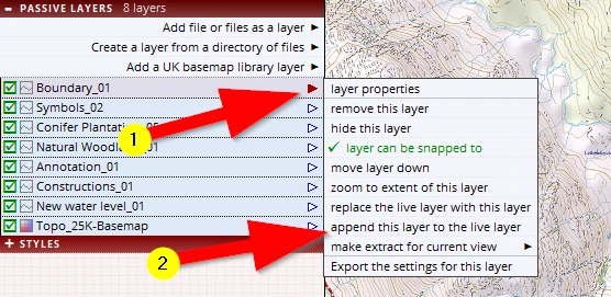
As the menu option name suggests, it adds information to the live layer, as opposed to clearing all that is in the live layer an replacing in it with something new (see option above it).

6.2 Adding layers

This is the first option in the PASSIVE LAYERS header (see image above Add file or files as a layer). As previously mentions, unlike software packages like Word or Excel, GIS software packages make use of many different file formats and thus the user must know which file type to look for. So, whenever we get a ‘Browse’ button to navigate to a folder, we must also filter out the file type. Many a novice map maker tends to forget this dual action (Folder and Filter type).

Creating, Adding and Removing layers is at the heart of map making and we will practise all this throughout the course, for example in the next paragraph!

6.3 Removing a layer

Now that the dam is established and the water level is rising, we are interested to know the maximum width of the new water level. Of course we can use the tape measure tool, but it could be we want to show this dimension on the map. For that reason (and for an exercise) we will not use the tape measure tool but draw a line and use that to measure the width.

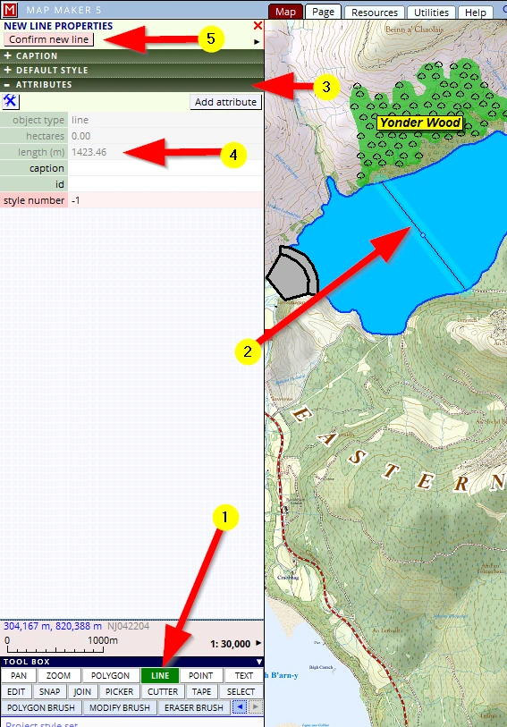
(1) Activate the LINE tool.

(2) One click on the shore, move the mouse to the other shore, click again, right mouse click to tell MM5 you are finished drawing.

(3) MM5 will open a new (green) menu on the left.

We are not interested in assigning a style, we only want to know the length. Open the ATTRIBUTES header.

(4) Here we can read the length of the line.

As mentioned, depending on how the map looks, we might decide to include this line in the final print, so we might as well save this as a layer.

(5) Confirm new line

We need to save this layer:

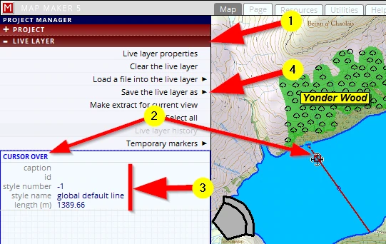
(1) It is a live layer, so the logical place to look for a menu to save this layer is in the ... LIVE LAYER header

(2) Below the menu options we see an empty grey section with the title CURSOR OVER

Please hover your mouse over the live layer object and ……

(3) ...note that MM5 will list all data which is on record

(4) Click on Save the live layer as and browse to the Training folder and give this file the name:

C:\MM_Course\Training\ Dimensions_01

The line is saved, but currently we do not want to have it as part of our map. Of course, this is only one line, but in other scenarios this layer could be an extensive survey with multiple polygons or lines which will just get in the way of drawing other things. In those cases we want to remove (or hide) a layer.

For the sake of practise we don’t want to hide this layer, we want to remove this layer from our map.

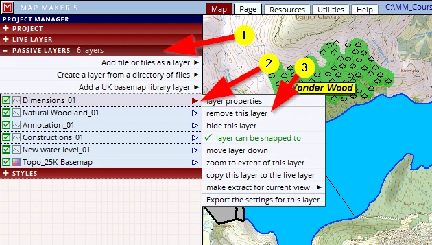
Because it is now a saved layer, the LIVE LAYER header is empty. Our work has now become a passive layer so we can expect to see this new layer in the PASSIVE LAYERS header:

(1) Open the PASSIVE LAYERS header

(2) Click on the little arrow after the layer name

(3) Select the option remove this layer

Since we have saved our layer, and physically did not change anything in the project, there is no need to save our project.

Bear this layer in mind as we will get back to this layer later on.

7 EDITING tools

7.1 The CUTTER tool

The cutter tool might be one of the newest tools in various software packages, but Map Maker introduced the cutter tool right off the bat when it was launched in the 1990s. It took other mapping/GIS software packages about 12 years to come up with the same...

The function of this tool is of course explained in the name, with this tool we can cut up a polygon into smaller sections.

It is often the fastest and best way to map the largest extent of an area first and then use the cutter tool to divide it up into smaller units.

Our conifer plantation is rather big. To make it more manageable, we will divide it into smaller management areas - compartments.

Looking in the PASSIVE LAYERS header, we see that:

The Conifer Plantation layer is the first layer in this stack. All other layers show in the sequence in which we created them. But this sequence of layers is ‘fluid’, it will change as we work in the project. We can select any vector layer in this stack and copy that into the live layer. When we copy a layer into the live layer it disappears from this list because live layers are always on top of all layers. When we save it, it will show up in the passive layer list, on top of all other layers. And thus the sequence of these layers will change during our work. Later in this project the sequence becomes important because it effect how the map looks.

(1) We need to work on this Conifer Plantation layer. A passive layer cannot be worked on, it has to be a live layer, so we need to copy it into the live layer. Click on that layer to select it

(2) Click on the little arrow after the name

(3) copy this layer to the live layer

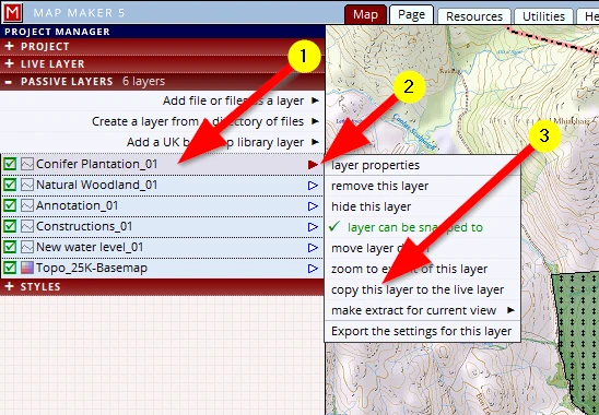
Note how this layer entry disappeared from the passive layer list. It is now a live layer and sits on top of the passive layers.

We now see a little blue dot in the centre of the polygon indicating it is in the live layer, ready to draw more polygons or edit it. We want to subdivide this polygon:

(1) Activate the CUTTER tool

(2) Click once on the boundary of a polygon to be split

(3) Click and trace the new boundary as you want it to be (please do a similar cut as shown below)

(4) Click on the opposite boundary and automatically the one polygon will have been split in two!

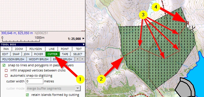
The one polygon has been cut in two and we can now also see two live layer dots.

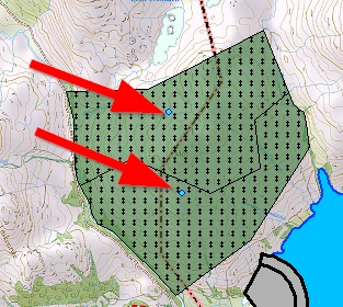
Please make one more cut, exactly like this, (close to and parallel to, but not on, the transmission line):

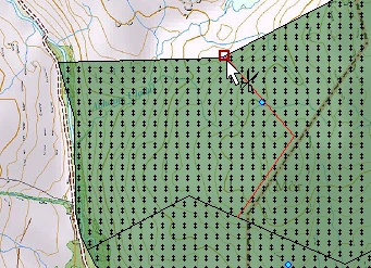
We will now save this live layer.

LIVE LAYER header, Save the live layer as, Conifer Plantation_02 in the training folder.

Which is an incremented version number (_02) Follow it up with an ‘F1’ to save the project.

Note that this layer now reappears in the PASSIVE LAYERS header, on top of the stack.

7.2 CUTTER tool options (e.g. buffer zone)

Transmission cables don’t run through woodlands like this:

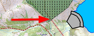
Note: If the transmission line does not show at all in the woodland, it is probably because you failed to set the fill opacity of the coniferous woodland style to 50%.

Usually an open space is created and maintained on either side of the cable. MM5 has specific functionality with regards to such ‘buffer zones’ and one of them is the following cutter tool setting:

Copy the layer back into the live layer: Select the layer, black arrow, Copy this layer to the live layer)

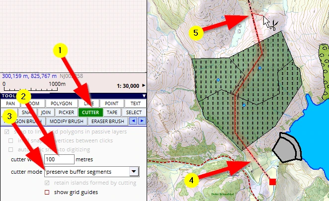
(1) Activate the CUTTER tool

(2) for the cutter width type in ‘100’

(3) with this setting we can decide what will happen with the created buffer. We will change it to preserve buffer segments for we want to explain more functionality after this. Do check out what other options are available

(4) In the previous cutter example we started ‘on’ the line and finished ‘on’ the polygon boundary again.

Just to show something different, we’ll now start ‘outside’ the polygon and will follow the transmission line, click, click, click on it.

Note: trace it as close as you can. Perhaps the cutter line even snaps automatically to it –depending on settings; we will explain those later).

(5) Note the red glow, indicating the cutter width. We will finish with a right mouse click outside the polygons to be cut.

After the right mouse click to finish the cut, we end up with this:

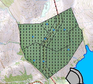
The corridor now consists of three different polygons, and they all have the plantation style indicating they are planted up. We need to do something about this. We need to change this style to something else. It should be ‘Open Ground’.

There are two ways forward to clear the transmission line through this woodland.

The first obvious one is that we simply delete the polygons which make up the corridor.

We don’t want to do that, because ‘Open Ground’ is part of the woodland and is valuable area in woodland management.

The second is that we assign a different style to it, showing no trees and a different colour. To do so we must first whip up a style which we will call ‘Open Ground’. Leave the live layer on screen.

Hit the ‘F2’ key on your keyboard. It will open up the style editor. Add a new style in the polygon tab, call it ‘Open Ground’ and leave the fill colour (a faint yellow) as is.

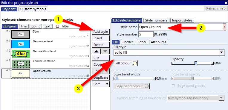
Hit the ‘F1’ key to save the project (and thus saving these changes to the style set) and close the style edit menu (white X top right).

Assuming we have the ‘Conifer Plantation_02’ still in the live layer:

Zoom in a bit to see what we are doing.

Change the style of one of the corridor polygons to ‘Open Ground’ (using the EDIT tool, click on it, go to the DEFAULT header and change the style).

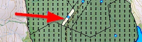
We could proceed and assign the Open Ground style number to the other 2 polygons as well.

But for the sake of explaining things we shall not. We will introduce some other useful tools, starting with …

7.3 The PICKER tool

In this simple example we only need to change a few polygons from one style to another, but imagine a big woodland where many compartments might have the same attribute data like Species, Plant year, Yield class, Spacing, Height etc. and of course the same colour on the map - the style. That is a lot of data to type up/change in each polygon.

The picker tool allows us to absorb attribute data from one object and carry it over onto the next. It is an immense timesaver to ‘populate’ your database and to change similar objects in no time.

In our little example we are only interested in carrying over the style:

(1) Activate the PICKER tool

(2) We have no specific ‘attribute data’, and the ID’s we will sort later, but make sure that the style number tick box is checked.

(3) Move your cursor over the polygon with the correct style and note how the cursor has changed into a little pipette, ready to soak up information.

(4) As mentioned before, note that the interface on the left, in the CURSOR OVER section, shows all that is on file for this particular object.

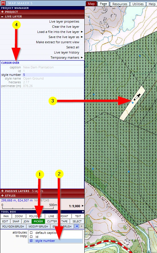
Then:

(1) Click, hold and drag to the next polygon and let go: that polygon will now have an identical set of information (and colour).

(2) Note that whilst you were moving the cursor to the next polygon, the interface changed colour indicating you have information ‘in’ the pipette.

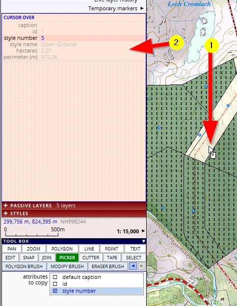
Now that you have information in the pipette, you can click on any other polygon (without having to absorb - click & hold). Just click on any other polygon you would like to change. Experiment with it with the other polygons (and change them back again).

We will only do the third polygon so it looks like this:

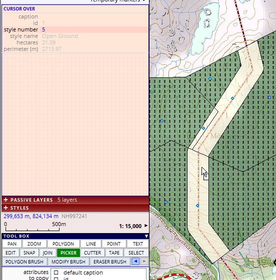
Remember: these were only 3 polygons, but in real life you may be dealing with many more and a lot more ‘attribute data’ and then this tool is super-efficient.

For the next exercise please change these three polygons back to what they were, the style and shape.

Let’s have a look at another tool which is also a very efficient one when it comes to dealing with multiple map objects in one go:

7.4 The SELECTION tool

The selection tool needs to know which layer it must work with, and so we first need to set that layer.

(1) Activate the SELECT tool

(2) Select the layer you want to work with. In this scenario it is the ‘live layer’.

Note: the SELECT tool has a double function, it can help you to edit work in the live layer but it can also interrogate data from a passive layer. When a passive layer is selected, the interface is colour-coded light brown, when the live layer is selected it is colour-coded blue (similar to that of the live layer dot).

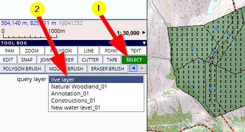
(1) When clicking on the little red/white question mark on the bottom left of the screen we can read how to make a selection - one single object, or multiple objects in one go, and different ways to do a multiple object selection (and how to de-select it):

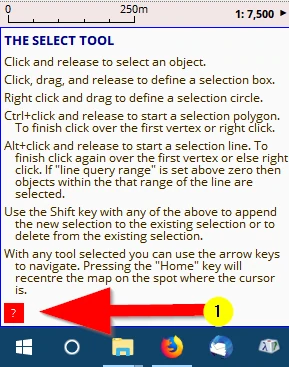
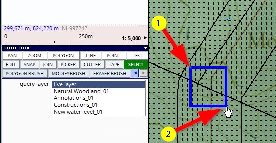
We want to select as many polygons as possible in one go. And zooming in a bit we realise we can select all three by dragging a selection box like so:

(1) Click & hold and drag the diagonal from the top left to the bottom right (like the zoom tool)

(2) Release the mouse button

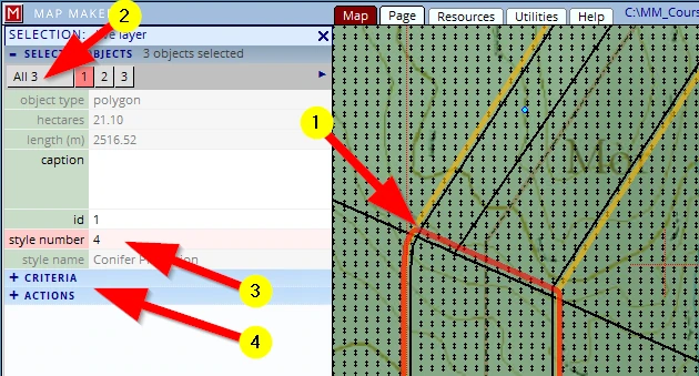
The interface on the left will have changed:

(1) In the map we can see which objects have been selected, they are highlighted with a coloured border.

And remember the instructions above, we can add and remove objects to this selection whilst holding down the keyboard ‘shift’ key when clicking).

(2) Currently all information of object 1 is shown. Click on the button ‘All 3’ so that we can make changes to all the selected objects - the interface will change slightly to accommodate this.

(3) In our scenario we only want to change the style number. Change it from ‘4’ to ‘5’ (= Open Ground’).

Job done!

But note:

(4) MM5 is a powerful GIS. In the CRITERIA header we can specify a simple or complex set of rules to make a selection and in the ACTIONS header we can perform all sorts of very efficient actions on these selected objects, but that is too much for this beginner’s course!

Because we clicked on the button ‘All 3‘ this new style number will have changed the style of all 3 polygons in one do to the new style.

As with many computer ‘selection’ tools (like selecting multiple files in a file browser), we can use the Ctrl or Shift key to add or remove from a selection.

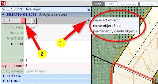
Please also check out the option in the submenu accessible by...

(1) clicking on the little blue arrow

(2) (which is only visible when one of the objects is selected)

Please leave this layer in the live layer.

Because of the cuts, we ended up with three polygons, all dealing with the open ground corridor.

What will follow is another tool which we can use to merge these three into one, using ...

7.5 The JOIN tool

We have used the cutter tool to subdivide the plantation and create the transmission line corridor.

The reverse action would be to join two adjacent polygons into one. We can do that using the JOIN tool:

(1) Activate the JOIN tool

(2) Click & hold in the polygon (which has a style and/or data you wish to expand):

(3) Move the mouse into another polygon to merge it with the first and let the mouse button go.

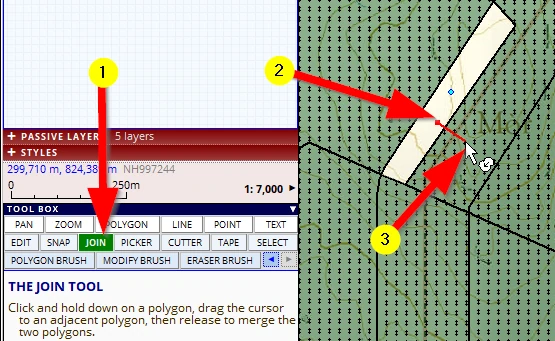
The two polygons become one.

We can do this again and we end up with one ‘corridor’ polygon:

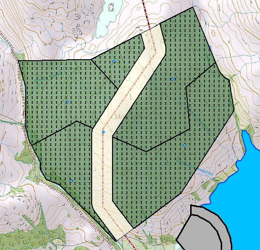
Note: On your screen you may see labels. We will deal with those later.

We have tried and done a lot. It is time save this layer with an increased version number (Conifer Plantation_03) and save the project (F1).

7.6 Deleting objects

We can get rid of unwanted objects in several ways. If you want to follow along, just draw several polygons somewhere, any shape and style will do:

One object

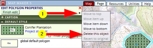
If one object needs to be deleted we can use the EDIT tool. Activate it and click once on the object to be deleted, then:

(1) Click on this little black arrow to open a new menu

(2) We can Delete this object in this menu. We can change the sequence of the objects, Move item up/down to get a specific cartographic effect if need be (we will explain and do this later).

Multiple selected objects

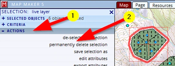
We can activate the Selection tool and drag a box around all and/or use the Ctrl or Shift key to add or remove items from this selection, then:

(1) click on the ACTIONS header

(2) click on the action: permanently delete selection

All objects in the live layer

(1) Click on the LIVE LAYER header

(2) Clear the live layer

Tiny objects

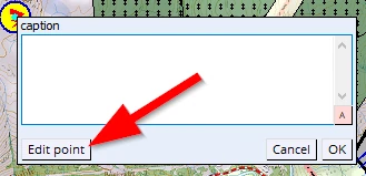
Very small objects can be difficult to select because often the label place holder is in the way. This is particularly true with symbols when the live layer label options are set to show a label.

With the Edit tool, click once on the symbol- the Edit caption menu opens, click on the button Edit point and the interface on the left opens as per usual to edit & delete the object.

Alternatively, make a selection with the Selection tool and deselect the unwanted object, then make use of the ACTIONS as described above.

7.7 The EDIT tool

We have used the EDIT tool a few times now. Let’s have a closer look at its functionality. In this section, please particularly focus on how the interface ‘talks’ to us (through e.g. subtle colour changes) using the tools.

With this tool we can physically change the shape of polygons and lines, add information to previously drawn map objects when that layer is in the live layer, and delete objects. After the tool is activated, a single click on any object will open the (green) menu headers on the left. Each header offers access to different aspects of the object.

But before we use the edit tool:

It has been decided to expand the plantation to the West with another new compartment. We need to draw that first with the POLYGON tool.

As mentioned, look closely how the software subtly ‘talks’ to us:

Please copy the Conifer Plantation layer into the live layer again and zoom out to about 50,000 scale.

Activate the POLYGON tool.

(1) Let’s start at the top and move the mouse over the boundary and as we move we give clicks to place vertices.

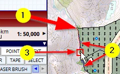
(2) As we move over the boundary of the polygon we see little yellow dots appear, on, before and after where the mouse is. This is an indication that there are vertices on those locations. If we were to click now, MM5 will snap the tool to the nearest vertex when not too far away.

(3) And if there is no vertex, but when we are close enough to an existing boundary, our cursor will also show a red square, indicating it will snap to the line.

Don’t zoom in, leave it at 1:50,000 scale as you draw. We will finish the new shape like so:

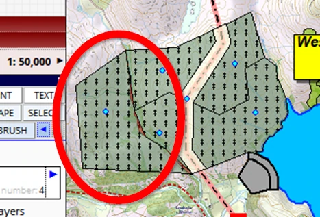
At 50,000 this looks like a nice extension to our plantation, we could now save the live layer (and project) and move on to do something else. However…

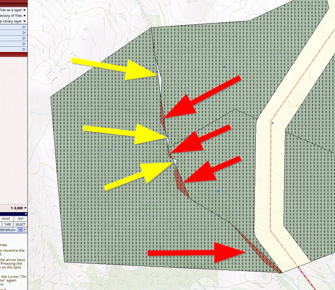
…when we zoom in to e.g. 10,000 scale we see that we have missed a few vertices and created gaps (yellow arrows). And we see that MM5 is highlighting overlaps (red arrows):

So far we have used the edit tool to change styles and change captions. We will now use it to amend the geometry of what we have drawn.

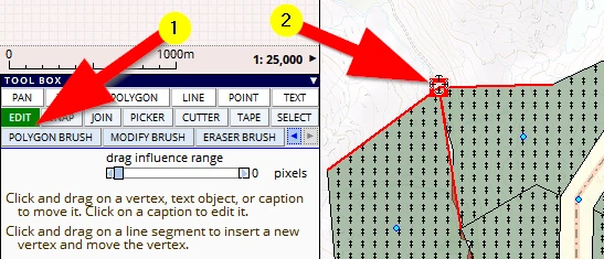
(1) Activate the EDIT tool

(2) Go to the starting point of our new polygon, and hover over this ‘T-junction’ of boundaries and observe that

a) The red square appears again, indicating we are over a vertex (i.e. a large square, a smaller square indicated we are over a line segment)

b) Three line segments turn red indicating that those are the three lines we will move together when we click, hold and drag this single point to a new location

When we hover the mouse over another boundary point of interlocking polygons: …

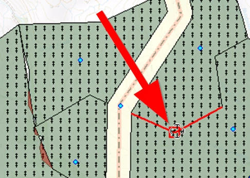
… we also see that the two line segments on either side are red, and so we can change the boundary of two polygons in one go.

This phenomenon of interlocking polygons is called …’Topology’.

On to the next session!