Session 9

Various

The following topics are beyond the scope of this beginners course, but even a few words might already open some more doors.

16 Useful extras

16.1 Gazetteers

We have drawn several things in several locations. During this course we have been zooming in and out on specific locations and needed to pan the image quite a lot to go to different sites. OK, this is a small map and covering a relatively small area, but think big. We may be dealing with a large area showing e.g. many farms or tenants or woodlands. To navigate from one site to the other can take quite some time (especially if your computer is not all that fast). Also, some other users of this digital map might not know where all these different sites are.

To help navigate to specific locations on the map we can set up a so-called ‘gazetteer’. A gazetteer is like a bookmark in your browser. It will allow us to mark a specific site and give it a name, after which this name appears in a ‘pick list’ so that the screen will automatically move to show this particular site at the scale we had it on screen when we saved the location in the gazetteer.

This is a very efficient navigation tool, a time saver and an aid for those not familiar with all the locations involved in a map. Furthermore, we can make good use of the gazetteer locations when it comes to printing multiple maps of the one site. Larger organisations or large estates will find this useful.

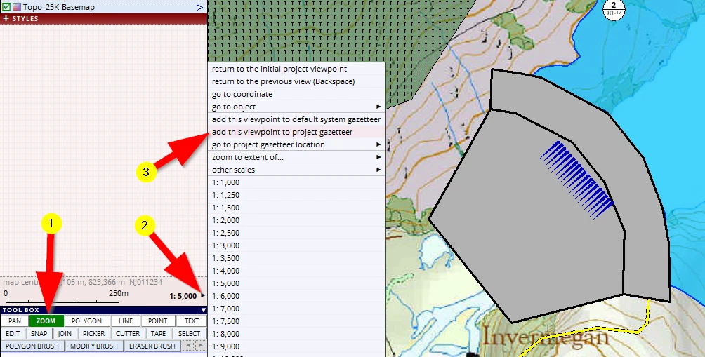
This is how it works:

(1) Activate the zoom tool and zoom in so that the dam is almost filling the screen

(2) Click on this little black arrow to open the next menu

(3) Activate the option add this viewpoint to project gazetteer

The interface changes, type in a name:

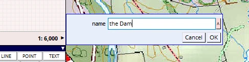
Do the same for some other sites, for example the new woodlands:

Yonder Wood, at 1:10,000 scale.

Conifer Plantation, at 1:35,000 scale etc.

Save your project (F1).

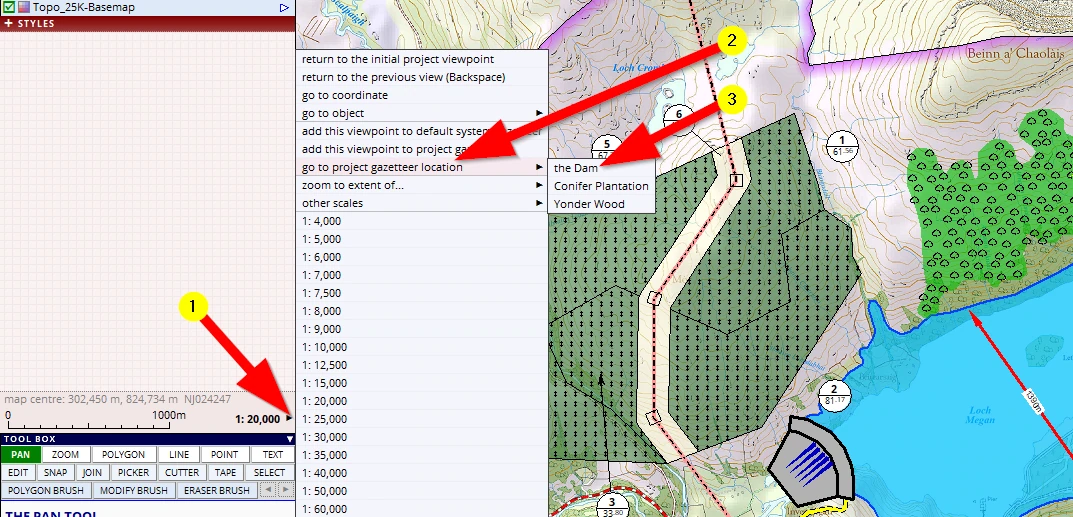
From now on we can quickly navigate to any of the saved locations:

(1) Open the navigation menu again and click on the new entry go to project gazetteer location.

(2) Click on a specific location and the screen will change to show the site at the same scale which it was when we saved this location in the gazetteer.

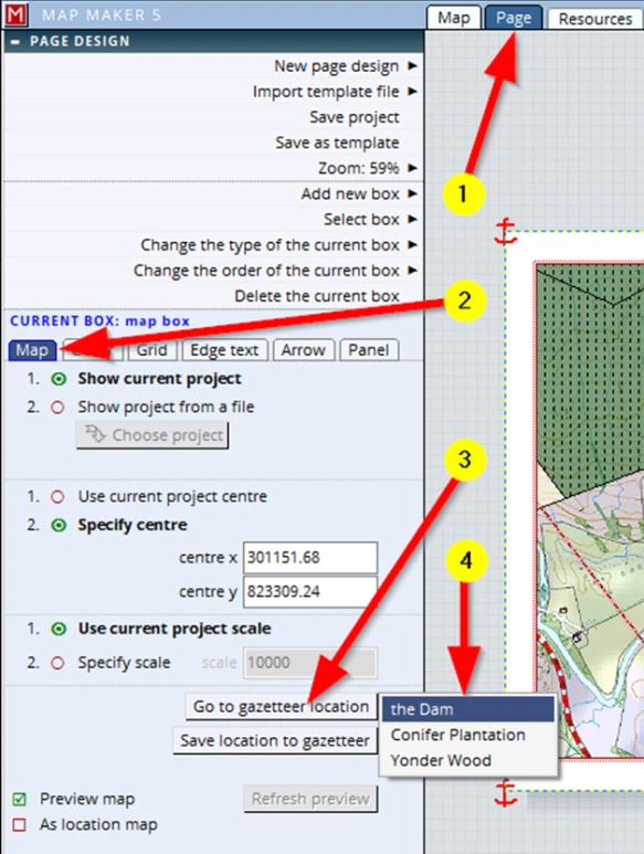
This gazetteer option can also be accessed in Page view which is handy when it comes to printing:

(1) Page view

(2) Click on the map box to activate the Map tab

(3) Go to a gazetteer location

(4) Select the location

Below this option we can also see the option Save location to Gazetteer which is handy to save a specific layout view. Call it e.g. ‘Print layout map centre’. So that whatever zoom, scale or view settings are active by activating this location, we can always quickly go back to a desired print layout.

Editing a gazetteer

We can also edit the gazetteer entries in the Resources tab.

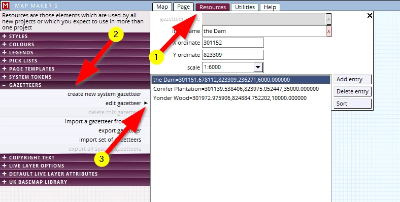
This might all be over the top for ‘one off’ map makers, but for larger organisations or large estates these are very powerful and efficient tools.

Advanced users and those in larger organisations will appreciate that we can also export the entries and import new data (which could have been created in Excel, or GPS data for example).

16.2 Markers

It is useful to know about ‘Markers’. What is a ‘marker’?

Well, think about working with paper maps. Suppose we need to set out a few measurements which for example were tape measured in the field, establishing a boundary. With the field notes and measurements next to the map, we would take out a ruler and set out the first measurement. We would then put a little ‘dot’ with our pencil to mark the spot, do the next measurement, again place a ‘dot’ and only then we would draw the line between those two measured dots. Those dots are temporary and we use a rubber to remove them.

MM5 offers a digital (but more useful) variant of this ‘dot’!

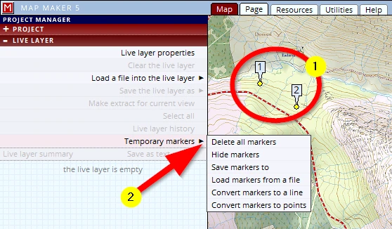
Please get your map on screen and move your mouse somewhere in the map. It does not matter what tool is active or what you are doing. Whenever the mouse is in the map view we can tap on the ‘m’ key on your keyboard. This will place a ‘Marker’ (1) !

Markers are in the live layer and in the LIVE LAYER menu we find a menu (2) with some useful options.

Although markers are temporary, they are saved when the project is saved and so will show up the next time we open this project again. In this menu we can delete them, hide them and save them (as ‘markers’), but we can also convert them to a line, which is then drawn from marker to marker (however many markers we placed). Alternatively we can convert the markers to symbols.

But there is more!

We can activate the EDIT tool (1) and click on the yellow dot (2). This will open a new menu.

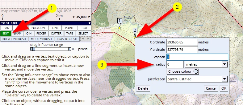
This menu is handy to e.g. copy and paste the coordinates from, or we can type in specific coordinates.

We can change the caption and colour etc. but we can also show a circle around this marker which is handy to reconstruct field measurements.

In the navigation menu:

we also find a go to marker option.

17 ATTRIBUTE data

Again, it is not in the scope of this beginners book to dive into all this, but no harm to add few words on ‘attribute data’.

What is ‘Attribute data’?

We have already ready seen the basics of this. When we draw a map object, the computer registers all sorts of additional data. For example it calculates and lists the area of polygons, the length of the perimeter. It can record a unique ID of any map feature and we can type in a name (Caption) and can assign a style number to it. That is computer related. However, a map is a 2D representation of real physical objects in the 3D world. All these objects will have lots of specific information which is also relevant to have on record.

For example:

Arboriculturalists may record in a tree survey:

tag number, species, condition, PofF, girth-width, age, risk, etc.

Ecologists may have done a heathland survey and would want to record e.g.:

survey date, the type of vegetation, health, wildlife seen on it, soil type, drainage.

Farmers would like to record e.g.:

crop, planting date, soil quality, applied fertilisation in an area.

Foresters are interested to know about e.g.:

species, plant year, yield class, thinning and felling phases, volume, tree heights.

Land Agents/Owners are interested in recording e.g.:

ownership (trusts), conveyance numbers, tenant details, rights, constraints.

In short, the usual stuff. In other words these are ‘Attributes’ of an object. This data can be ‘Attributed’ to the drawn map objects.

In several places in the interface we have seen the ATTRIBUTES header. For example, when we draw a new object, edit an existing one or select an object(1). As mentioned: the software automatically records some default information as can be seen in the highlighted section (2).

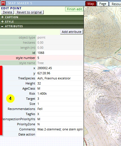
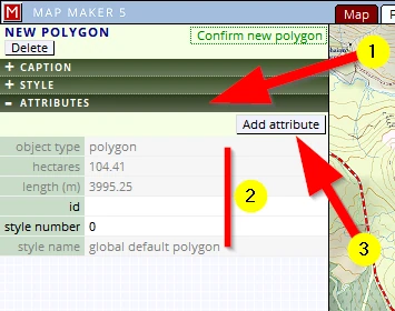
We can add our personal records here (3), which then show up here (4).

This type of data usually lives in a Spreadsheet somewhere. Well, Map Maker has that too. It is part of the drawing.

(1) It can be viewed in the layer properties menu (and this can be accessed in the live layer settings or the passive layer settings)

(2) Attributes header

(3) The first few entries (marked red) are the default entries (Object type, Ha, Style, Caption etc.)

(4) The following columns (marked green) are introduced by the user.

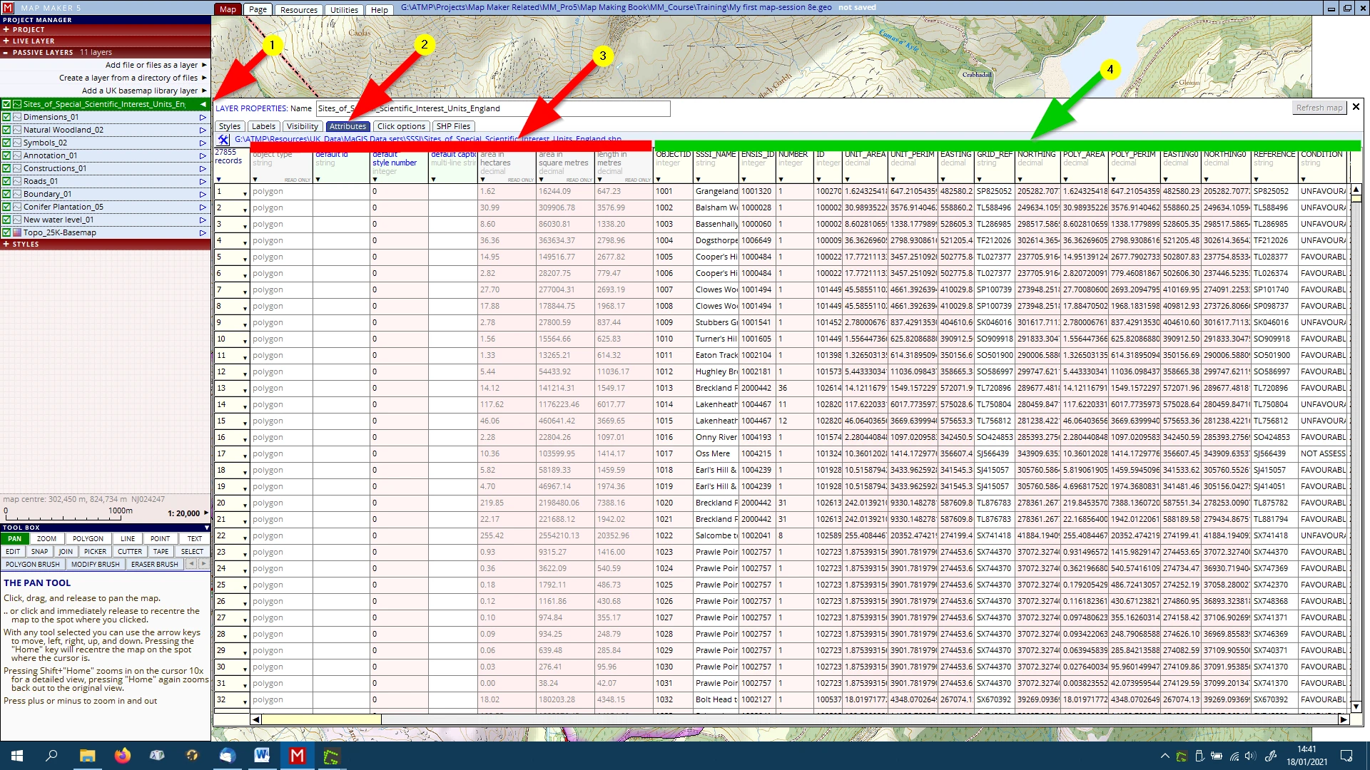
(There are scroll bars to the right hand side and bottom to scroll through long and wide records.)

And just like a spreadsheet, one can do all sorts with this data.

(1) Click on the little arrow in the column header...

(2) …and see and explore what can be done with it all.

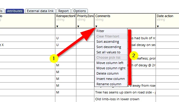
The above data is kept in the MM5 dra file. Naturally MM5 allows us to link to external databases as well (e.g. a MS Excel spreadsheet). Each map object should have a Unique ID which can also be found in this external database. The interface will guide you through this linking process.

As mentioned, this is all advanced stuff and there is too much to explain in this course, but there you have it...

18 RESOURCES & UTILITIES

The interface explains the function of these tabs:

The functionality of the tools in these sections are very useful and powerful. Some of these tabs will be used by many map makers, beginners or advanced users (we already used the ‘Legend Editor’). Other tabs only will come into their full right when the software is used in a larger organisation. Some options are typical tools for when the software is more used as a Geographic Information System (GIS) as opposed to drawing a map. All in all, these two make up a very complete toolbox for novice and advanced users - no harm exploring some options.

Below are a just a few ‘Utilities’ examples. When activating any of these tool we will first be asked which file to use.

• When labels of polygons for some reason have been moved about but should all show in the centre of each polygon:

Utilities, VECTOR, Amend labels, ensure polygon labels are inside

Check out the other label actions too!

• When an old map has been scanned and needs to be inserted into a project as a layer:

Utilities, BITMAPS, calibrate bitmap

• On the internet there is a lot of useful data available which can be inserted directly into MM5 as a layer, reading the data off an internet based supplier (e.g. the Forestry Commission, also, see Appendix A4):

Utilities, WEB MAP SERVICES

• Many use Excel. These spreadsheets can be linked to a MM5 drawing. However, it is often useful to physically import and export data into the drawing, to speed up work. Check out the options here:

Utilities, DATABASES

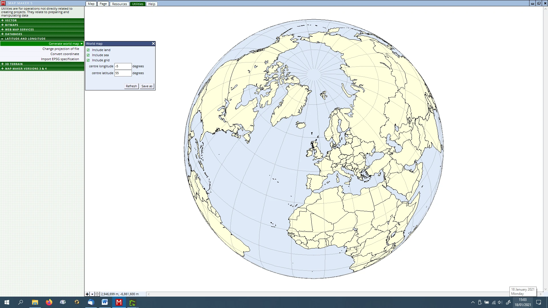
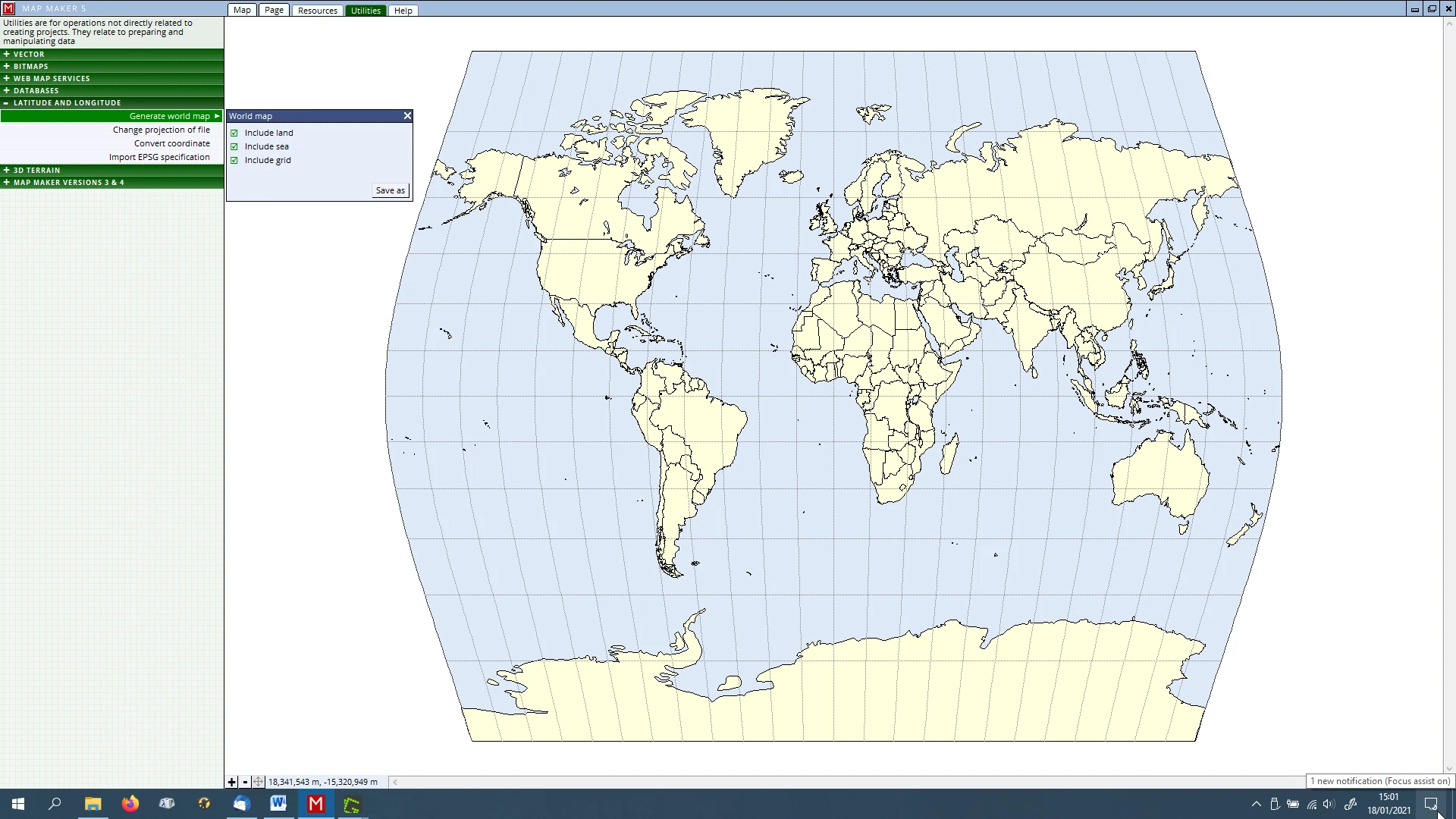
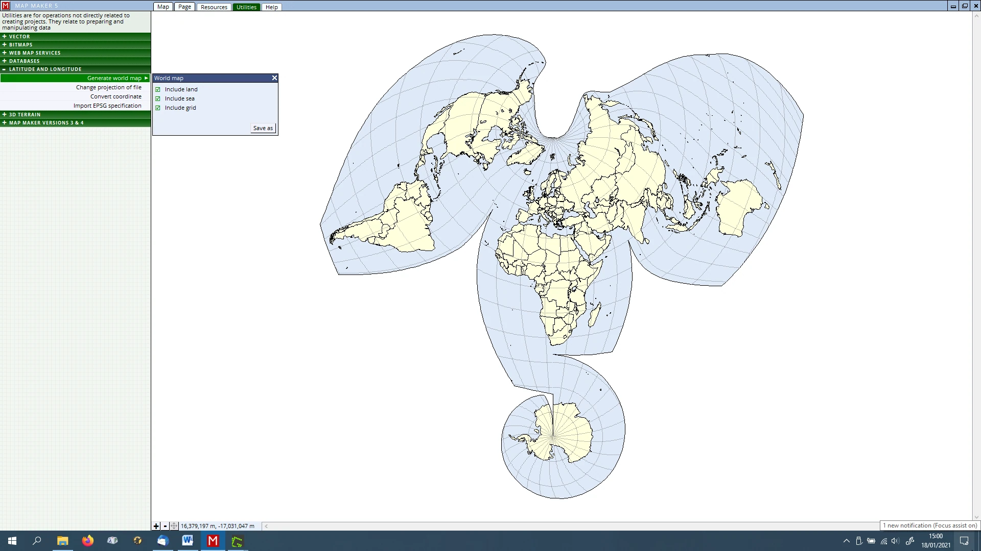
• Need a world map? Or need to convert raw Longitude/Latitude data into a particular map projections:

Utilities, LATITUDE & LONGITUDE (see images below)

• In need of contours, hill shading or altitude colouring?:

Utilities, 3D TERRAIN

• Of course MM5 can open and work with data from previous versions without much further action to take. But here are some tools to convert old data into this new and better MM5 format.

Utilities, MAP MAKER VERSIONS 3 & 4

19 IMPORTING & EXPORTING data

19.1 Importing data

There is a lot of useful data out there ready to be used in our projects. For example:

• organisations like Local Authorities may be flexible enough and willing to exchange e.g. their Public Rights of Way map layer.
• Utility companies may be willing to exchange their overhead and underground cables and pipe map layers
• Scottish Natural Heritage, Natural England and e.g. the Forestry Commission also have a lot of useful data.

MM5 can import most industry standard file formats. The importing process and associated menus are easy and self-explanatory.

However, a few words on the two most common exchange file format might not be amiss. Then we will put it into practice in our map:

ArcVIEW SHAPE files

It is important to realise that ArcVIEW (a part of the ArcGIS software suite) deals with data in a slightly different way from Map Maker. With MM5 when we save a drawing, it is one file. The database is part and parcel of it. When saving the same layer in ArcGIS we end up with three files and some users even expect to see a fourth file.

The files are: *.dbf, *.shp, *.shx and the fourth one is the file which contains the projection data: *.prj

In other words, when it comes to exchanging data, always make sure you end up with this triplet of files. If one is missing things will not work.

Because ‘Shape files’ are the undisputed industry standard, MM5 can read and write effortlessly with these files. There is no import or export required, we just open the layer, copy it into the live layer and save it again as a *.SHP file. So far we have just saved all our work by giving it a name, and by default MM5 saved it as a *.dra file. But in that same menu we can also choose to save it as a *.shp file. That is done here:

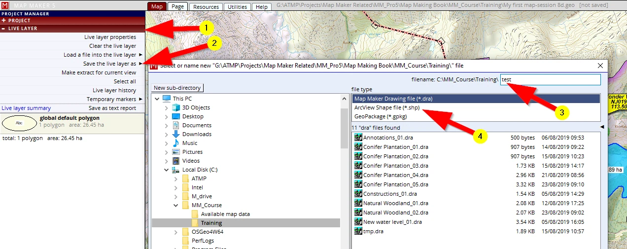
As mentioned, save it as a MM5 *.dra file and we end up with one file, save it as a *.shp file and we end up with 4 files!

Furthermore, in MM5 we can draw all map objects in one layer (polygons, lines, points and text) but ArcVIEW only accepts one object type per file. So that means we could potentially end up with 16 files where MM5 deals with it in one. For that reason MM5 will not allow you to save it as a SHP file when there are different object types in one layer. If that is the case, we need to save it into a *.dra file first, then we need to use the EXPORT function (see next section).

MapINFO files

MapINFO is another GIS software package commonly in use: the one layer will be exchanged in two files. A so-called *.MIF and *.MID file.

If one of these two is missing, an import will not work.

There are other file formats we may come across, like importing recordings from our GPS kit for example, or polygons which we drew in Google Earth. We can import a range of the most common industry standards here:

(1) Utilities

(2) VECTOR

(3) Import vector file

(4) Click on the little black arrow to open the final menu listing showing all possibilities.

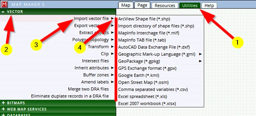
Each import will open up different menus depending on the type of data. It is quite obvious what options to choose and which ‘OK’ buttons to click.

A final note:

When exchanging drawings like this, it is important to realise that GIS packages only exchange the ‘raw’ drawing: the actual line work with the associated attribute data. The styling of this data, the colours, lines, fonts symbols etc. is software specific and is therefore often not exchanged. This means that all this type of exchanged data must be reviewed, then the GIS users (of whatever software package) must create styles for the objects in it. If we fail to do that, GIS software which opens such data will just display this raw data with some bland ‘default’ styling.

19.2 EXPORTING data

The reverse of importing data is of course Exporting data. Read what was said regarding importing data, all that applies to Exporting data as well. The Export options can be found in the Utilities tab. The interface will make it quite clear what steps to take.

20 CARTOGRAPHIC EFFECTS

20.1 Masks

A face mask covers a face. A cartographic mask covers an area, so if we want to apply this cartographic effect we need to have polygons ready which can act as a mask.

Here is an example of typical use:

We already mentioned that we felt our map shows quite a lot of information and our eyes tend to wander to and fro over the map. We want to tell a specific story with this map and want to draw attention to our specific project/information. In other words, the coloured Base-map outside our project area is interesting (to show the context), but effectively it also offers a lot of visual input which distracts from our specific information.

This is where a ‘mask’ comes in handy. It is useful to show the context, but all those colours outside our project area are just too much.

Let’s apply a mask!

We want our map readers to focus on our project area. Therefore the obvious choice for a mask is to use the file ‘Boundary_01’.

Try the following:

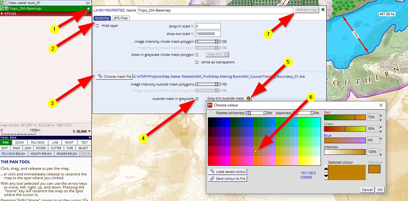
(1) Select the ‘Topo_25K-Base-map’ and open the layer properties

(2) It will have opened on the Visibility header

(3) Click on Choose mask file and browse to our Training folder and select the ‘Boundary_01 ‘ file.

(4) Tick the box outside mask in grey scale.

Leave this menu open and click on Refresh Image (7) and see how all the colours outside our project area are now in grey. That is too grey for our liking so we will experiment with the option...

(5) ...Grey tint outside mask, and choose

(6) this light brown and OK this menu away

(7) Refresh again to see the effect

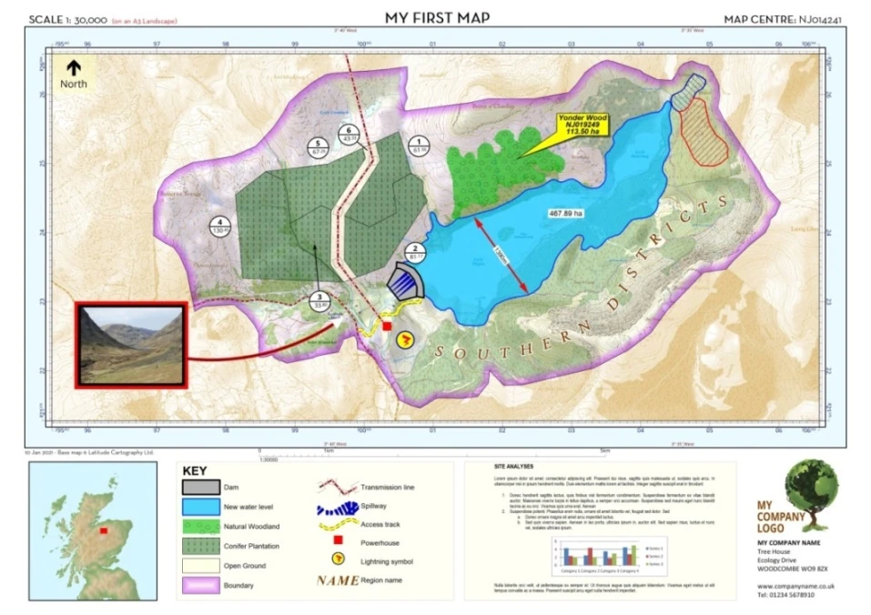
Although this is a very slick effect and our eye is instantly draw into our project area, we think in this case we do like to see at least some context colours.

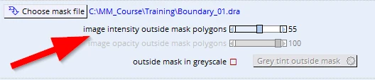
So back in the layer properties, Visibility header we uncheck the greyscale option and adjust the slider reading image intensity outside mask polygons to back to about 55%.

20.2 Duplication of layers

It was mentioned that one of the reasons to create different layers is to get specific cartographic effects. Below is a typical forestry example which makes good use of layers. The principles involved can easily be applied in other scenarios as well.

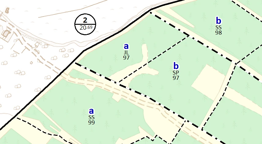
• The label information shown (e.g. ’a’ and ‘SS 99’) is created by introducing the same layer twice as a passive layer. The first layer shows the Sub-CMPT letters in bold blue. The second (same) layer, shows the Species and Plant year, but in a smaller font and in black. The labels in the second layer are moved down (in the Layer properties, Visibility header).
• The Boundary is a 0.5mm line, the CMPT boundary 0.4mm and the sub layer is 0.3 mm, thus the hierarchy and sequence of layers suppresses one over the other to get this visual result.

20.3 Assigning styles

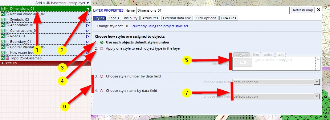
We can see the various options how to assign styles in this menu:

(1-2) Open the LAYER PROPERTIES menu (either in a passive layer or live layer)

1. Using the style number in an object

When we draw or edit objects in the live layer we can assign a style number to each individual object. That number is now part and parcel of the data kept in the Drawing file. By default MM5 uses the first option: Use each objects default style number (3).

2. Apply one style to each object in the layer

Sometimes all objects in a layer need to have one particular style. After we have selected this option (4) we must specify which object types we have in mind to alter, and then choose a relevant style for these objects (5). Regularly when drawing and editing, colours and styles get in the way. This option offers a quick change. Also when we use e.g. SHP files, we can apply these style settings.

3. Assign a style by using a database entry

GIS map layers usually have a lot of associated data e.g. field names, ownership codes, species, plant years, felling phases etc.

With these two options (6) MM5 allows us to tap into such data. Once selected we need to specify in which data column our data lives (7).

The first option expects an integer as an input field. Such a number must have a matching style number in the style file.

The second option expects a text. MM5 will then match this text with an identical text which we can type in as the style name in our style file.

20.4 Advanced use in action!

In the previous chapters we have explained some advanced stuff even though this is a beginner course. For the adventurous, let’s try to see this in action!

Our ecologist came in to discuss his findings and mentioned that in the north of our project area there is a ‘Site of Special Scientific Interest’ (SSSI) which should show on the map. He sourced the relevant polygons from the National GIS open access dataset and handed over the ArcView SHAPE files of these and told us there are two different ‘types’ to show.

We can find these *.SHP files in the ‘Available map data folder’. Checking the folder with Windows Explorer we indeed see 4 files all bearing the same name: SSSI.*

As mentioned a few times: MM5 can work with SHP files without the need to import that data and convert it to MM5 native DRA file format.

In the PASSIVE LAYERS header we see the option, Add file or files as a layer. We need to select the file type ArcView Shape file (*.shp) and when it is on screen we can see them in a system default colour (4).

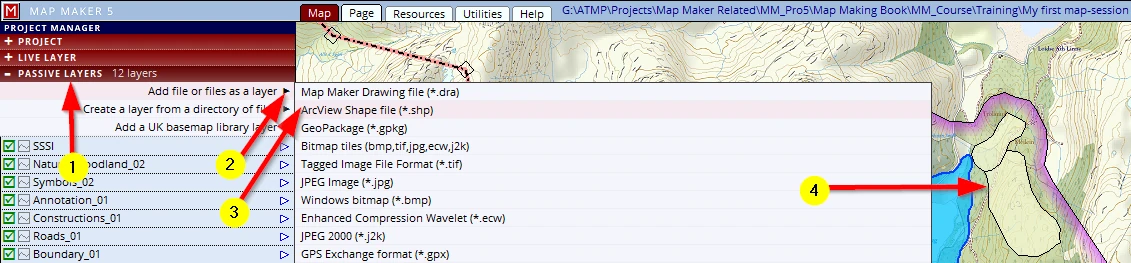
The reason they show up in this yellow tint is because we do not have a style ready for it and the software does not know which style to assign to these polygons. This is ‘raw’ GIS data: we need to take charge of the styling.

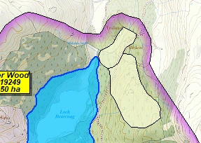
We can add the SHP file as a layer into our project and we note they show up with a default style:

We select that passive layer, open the layer properties menu and access the Attribute header (1-3).

There we see an impressive range of data columns. We were informed that the ‘type’ is of interest (whatever that means). Indeed we find a column with a header called ‘TYPE’.

We see this column only has two entries and each entry has got one of two entries: MIXED and BIOLOGICAL.

So far we have learned that MM5 uses style numbers, to assign a style to map object. This column has got ‘text’ to make a class/style distinction.

MM5 helps out - there is an option so that we can use these text entries to assign a style.

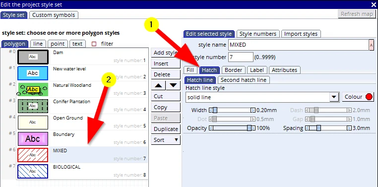
The way forward is this - we need to create two styles, each should have exactly this text as a style name. MM5 will then be able to read the values in this column and assign the style which has the same name as that data entry.

F2 opens the style editor and we can create two new styles: one with a red hatch (named MIXED) the other a blue hatch (named BIOLOGICAL). We need to set the Fill type to left or right sloping hatch and the fill Opacity to 0%, then we can go to the Hatch tab too. It is only once a fill hatch type is selected that we will see more tabs to tweak the colours, thickness and spacing (1) so that the results looks like this (2).

It is crucial that the style name is identical to those found in the column we are interested in.

Save project (F1) to save these new style additions.

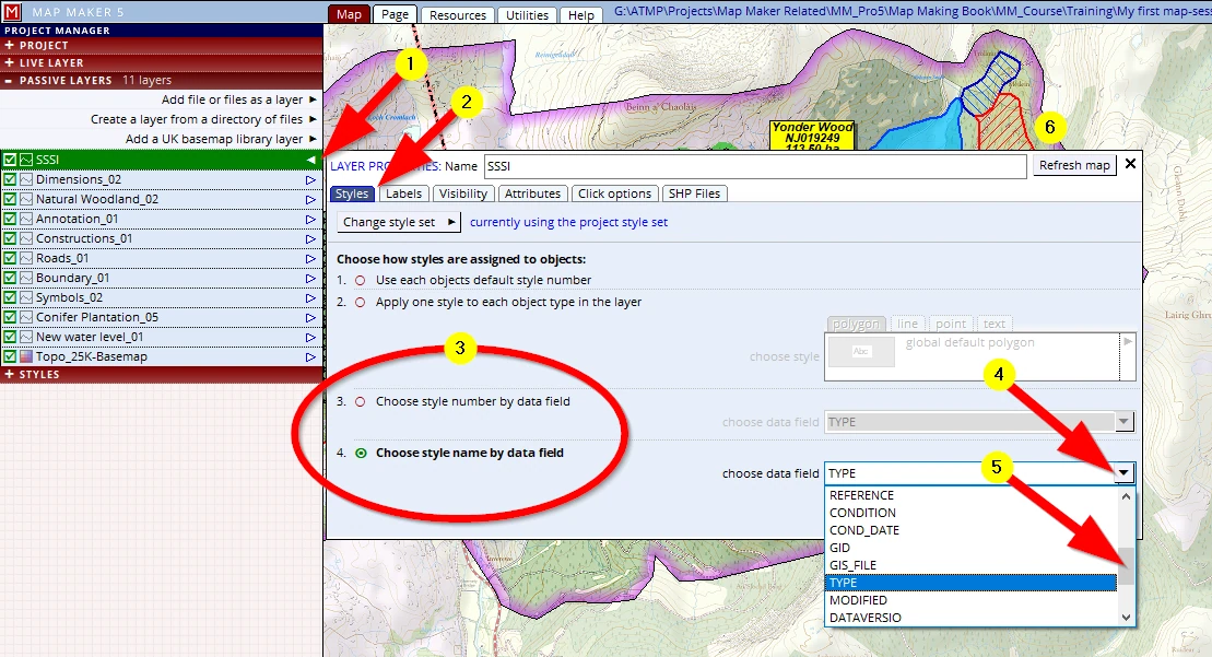
(1) Select the SSSI layer and open the layer properties menu

(2) In the Styles header we see four options to assign style numbers

So far we have used the default option 1. Use each objects default style number.

For the Dimension line we used option 2. Apply one style to each object type in the layer

(3) The last two options will read columns from the attribute table.

Option 3. Choose style number by data field assumes a number (and integer) in the selected column so that MM5 will use that integer as its style number.

The next option, 4. Choose style name by data field will use the given text and will match that with a style carrying the same name

(4-5) We will scroll down and select the ‘TYPE’ column

(6) When we refresh the screen we see that the styles have been applied

F1 to save your project!

20.5 Template paper size change

If all is well, by now our map should look like this:

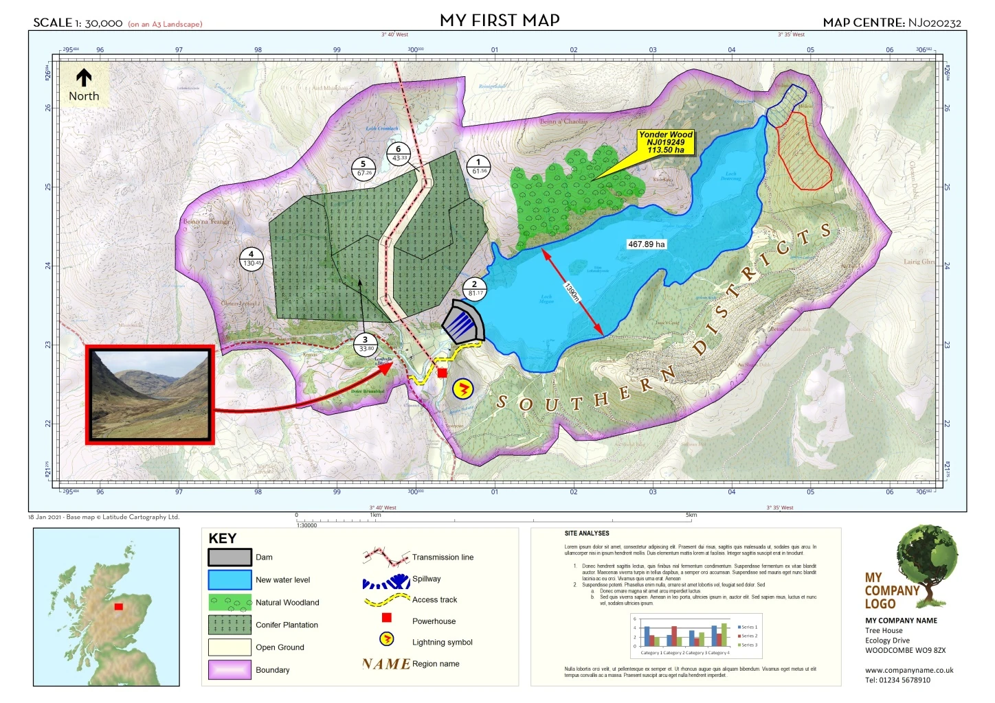
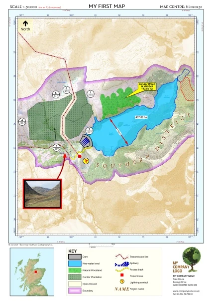
We have designed our map to be an A3_Landscape. Let’s create a new map, the very same but now to print it out A3_Portait. This would constitute the creation of a new map, based on a previous project we made. So in line with what we have taught:

• Open the previous project.
• Instantly do a Save project as, and name it: My First Map-Session 9_A3-P

Then go to the Page tab and open the PAGE DESIGN header (or click once in the grey outside the page). Change the Paper size to A3 Portrait.

Provided we took care of all the anchor points when placing the template boxes, the new layout should neatly jump into line. The only logical exception is of course the Legend box and the MS word box - they are both quite wide and we simply do not have the width of paper anymore to show both. We need to make a choice which to show and with some minimal adjusting we could end up with something that looks like this:

21 CONCLUDING

This concludes this map production. We hope you have enjoyed this course and that you will be able to apply it in your daily work!

As with most things we have learned in life:

“If you don’t use it you will lose it”

It is quite possible you will not use this software and these skills daily. When you get back to it after a while and need to refresh your memory, please read Appendices A1 & A2. They are intended to do just that, a very brief reminder of the crucial concepts involved.

Happy mapping!